
Covariance and Correlation
Covariance and correlation are the two key concepts in Statistics that help us analyze the relationship between two variables. Covariance measures how two variables change together, indicating whether they move in the same or opposite directions.
 Relationship between Independent and dependent variables
To understand this relationship better, consider factors like sunlight, water and soil nutrients (as shown in the image), which are independent variables that influence plant growth our dependent variable. Covariance measures how these variables change together, indicating whether they move in the same or opposite directions.
What is Covariance?
Covariance is a statistical which measures the relationship between a pair of random variables where a change in one variable causes a change in another variable. It assesses how much two variables change together from their mean values. Covariance is calculated by taking the average of the product of the deviations of each variable from their respective means. Covariance helps us understand the direction of the relationship but not how strong it is because the number depends on the units used. It’s an important tool to see how two things are connected.
- It can take any value between - infinity to +infinity, where the negative value represents the negative relationship whereas a positive value represents the positive relationship.
- It is used for the linear relationship between variables.
- It gives the direction of relationship between variables.
Covariance Formula
1. Sample Covariance
CovS(X,Y)=1n−1∑i=1n(Xi−X‾)(Yi−Y‾)
CovS
(X,Y)=n−1
1
∑i=1
n
(Xi
−X
)(Yi
−Y
)
Where:
- Xi
- Xi
- : The ith
- ith
- value of the variable X
- X in the sample.
- Yi
- Yi
- : The ith
- ith
- value of the variable Y
- Y in the sample.
- X‾
- X
- : The sample mean of variable X
- X (i.e., the average of all Xi
- Xi
- values in the sample).
- Y‾
- Y
- : The sample mean of variable Y
- Y (i.e., the average of all Yi
- Yi
- values in the sample).
- n
- n: The number of data points in the sample.
- ∑
- ∑: The summation symbol means we sum the products of the deviations for all the data points.
- n−1
- n−1: This is the degrees of freedom. When working with a sample, we divide by n−1
- n−1 to correct for the bias introduced by estimating the population covariance based on the sample data. This is known as Bessel's correction.
2. Population Covariance
CovP(X,Y)=1n∑i=1n(Xi−μX)(Yi−μY)
CovP
(X,Y)=n
1
∑i=1
n
(Xi
−μX
)(Yi
−μY
)
Where:
- Xi
- Xi
- : The ith
- ith
- value of the variable X
- X in the population.
- Yi
- Yi
- : The ith
- ith
- value of the variable Y
- Y in the population.
- μX
- μX
- : The population mean of variable X
- X (i.e., the average of all Xi
- Xi
- values in the population).
- μY
- μY
- : The population mean of variable Y
- Y (i.e., the average of all Yi
- Yi
- values in the population).
- n
- n: The total number of data points in the population.
- ∑
- ∑: The summation symbol means we sum the products of the deviations for all the data points.
- n
- n: In the case of population covariance, we divide by n
- n because we are using the entire population data. There’s no need for Bessel’s correction since we’re not estimating anything.
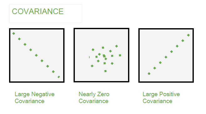
Types of Covariance
- Positive Covariance: When one variable increases, the other variable tends to increase as well and vice versa.
- Negative Covariance: When one variable increases, the other variable tends to decrease.
- Zero Covariance: There is no linear relationship between the two variables; they move independently of each other.
Example
 What is Correlation?
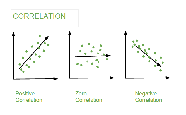
Correlation is a standardized measure of the strength and direction of the linear relationship between two variables. It is derived from covariance and ranges between -1 and 1. Unlike covariance, which only indicates the direction of the relationship, correlation provides a standardized measure.
- Positive Correlation (close to +1): As one variable increases, the other variable also tends to increase.
- Negative Correlation (close to -1): As one variable increases, the other variable tends to decrease.
- Zero Correlation: There is no linear relationship between the variables.
The correlation coefficient ρ
ρ (rho) for variables X and Y is defined as:
- Correlation takes values between -1 to +1, wherein values close to +1 represents strong positive correlation and values close to -1 represents strong negative correlation.
- In this variable are indirectly related to each other.
- It gives the direction and strength of relationship between variables.
Correlation Formula
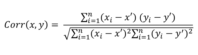 Here,
Here,
- x' and y' = mean of given sample set
- n = total no of sample
- xi
- xi
- and yi
- yi
- = individual sample of set
Example
 Difference between Covariance and Correlation
This table shows the difference between Covariance and Covariance:
CovarianceCorrelationCovariance is a measure of how much two random variables vary togetherCorrelation is a statistical measure that indicates how strongly two variables are related.Involves the relationship between two variables or data setsInvolves the relationship between multiple variables as wellLie between -infinity and +infinityLie between -1 and +1Measure of correlationScaled version of covarianceProvides direction of relationshipProvides direction and strength of relationshipDependent on scale of variableIndependent on scale of variableHave dimensionsDimensionless
They key difference is that Covariance shows the direction of the relationship between variables, while correlation shows both the direction and strength in a standardized form.
Applications of Covariance and Correlation
Applications of Covariance
- Portfolio Management in Finance: Covariance is used to measure how different stocks or financial assets move together, aiding in portfolio diversification to minimize risk.
- Genetics: In genetics, covariance can help understand the relationship between different genetic traits and how they vary together.
- Econometrics: Covariance is employed to study the relationship between different economic indicators, such as the relationship between GDP growth and inflation rates.
- Signal Processing: Covariance is used to analyze and filter signals in various forms, including audio and image signals.
- Environmental Science: Covariance is applied to study relationships between environmental variables, such as temperature and humidity changes over time.
Applications of Correlation
- Market Research: Correlation is used to identify relationships between consumer behavior and sales trends, helping businesses make informed marketing decisions.
- Medical Research: Correlation helps in understanding the relationship between different health indicators, such as the correlation between blood pressure and cholesterol levels.
- Weather Forecasting: Correlation is used to analyze the relationship between various meteorological variables, such as temperature and humidity, to improve weather predictions.
- Machine Learning: Correlation analysis is used in feature selection to identify which variables have strong relationships
Calculating Covariance and Correlation
Last Updated : 24 May, 2025
Covariance and correlation are two statistical concepts that are used to analyze and find the relationship between the data to understand the datasets better. These two concepts are different but related to each other. In this article we will cover both covariance and correlation with examples and how these concepts are used in data science.
Covariance
Covariance measures how two variables change together indicating the direction of their linear relationship. To understand this, think of features as the different columns in your dataset, such as age, income, or height, which describe various aspects of the data. The covariance matrix helps us measure how these features vary together—whether they are positively related (increase together), negatively related (one increases while the other decreases), or unrelated.
The value of covariance can range between −∞to∞
−∞to∞ . It gives insight whether the variable is positive , negative or no relation.
- Positive covariance suggests that as one variable increases, the other tends to increase, while a negative covariance indicates an inverse relationship.
- Zero Covariance- when two variables are not related with each other and don't have any impact on each other.
However, covariance is not standardized, meaning its value depends on the scale of the variables, making it less interpretable across datasets.
The formula for calculating covariance between two variable (X) and (Y) is given below:
 where
where
- Xi
- Xi
- : Represents the ith value of variable X.
- Yi
- Yi
- : Represents the ith value of variable Y.
- N: Represents the total number of data points.
While covariance is useful to determine the type of relationship between variables but it is not suitable to interpret the magnitude of the relationship as it is scale-dependent, meaning covariance shows if two variables move together but because it depends on the units of measurement its value doesn't clearly indicate how strong the relationship is.
Now, when we need to understand the relationships between multiple features in a dataset, we use covariance matrix which is a square matrix where each element represents the covariance between a pair of features. The diagonal elements of the matrix capture the variance of individual features, while the off-diagonal elements indicate how pairs of features vary together.
The covariance matrix also plays a key role in feature selection and feature extraction by identifying redundant or highly correlated features that may introduce noise or multicollinearity into models. For example, highly correlated features can be removed to improve model interpretability and reduce overfitting.
Correlation
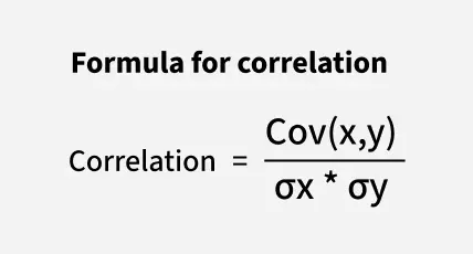
In covariance we find the relationship between variables but it doesn't find the strength of the relation. This problem is resolved by correlation. So It is a standardized version of covariance that measures both the direction and strength of the linear relationship between two variables by dividing covariance by the product of the standard deviations of the variables.
This results in a dimensionless value ranging from -1 to +1, where values close to +1 or -1 indicate strong positive or negative linear relationships, respectively, and 0 implies no linear relationship. The diagonal of the matrix always contains 1s, as each feature is perfectly correlated with itself.
The formula of correlation is given below:
 Where,
- Cov(X, Y): Represents the covariance between variables X and Y.
- σX
- σX
- : Represents the standard deviation of variable X.
- σY
- σY
- : Represents the standard deviation of variable Y.
we can classify the correlation into three types:
- Simple Correlation: It measures the relationship between two variables with one number.
- Partial Correlation: This helps to show the relationship between two variables while removing the influence of a third variable.
- Multiple Correlation: It is a technique that uses two or more variables to predict a single outcome.
Correlation is particularly useful for comparing relationships across different datasets or features in machine learning.
The correlation matrix is particularly useful for feature selection and exploratory data analysis. By identifying highly correlated features, data scientists can detect redundancy in the dataset and decide which features to keep or remove. For example, in regression models, eliminating highly correlated features helps avoid multicollinearity, which can distort the model's predictions. Additionally, the matrix provides insights into which features are most influential for predicting the target variable.
Difference Between Covariance and Correlation
Aspect
Covariance
Correlation
Definition
Measures how two variables vary together, indicating the direction of their linear relationship.
Measures both the relationship and strength of two variables
Unit Dependency
Units depend on the product of the units of the two variables.
Unitless, making it easier to compare across datasets or features.
Range
lies between −∞to∞
−∞to∞
lies between -1 and 1.
Methods of Calculating Correlation
The Graphic Method and Scatter Plot Method are simple, visual ways to understand correlation between variables
1. Graphic Method: In this method, the values of two variables are plotted on a graph, with one variable on the X-axis and the other on the Y-axis.
- By observing the trend of the plotted points:
- An upward trend (from bottom-left to top-right) indicates a positive correlation.
- A downward trend (from top-left to bottom-right) indicates a negative correlation.
- However, this method only gives an idea about the direction of the relationship and does not provide any information about its magnitude or strength.
2. Scatter Plot Method: A scatter plot is a more detailed version of the graphic method, where individual data points are plotted on a graph.
- Observing the arrangement of points:
- If the points form an upward pattern from left to right, there is a positive correlation.
- If they form a downward pattern from left to right, there is a negative correlation.
- If there is no discernible pattern, it suggests no correlation.
- Scatter plots are widely used in exploratory data analysis because they visually highlight relationships, outliers, and trends in data.
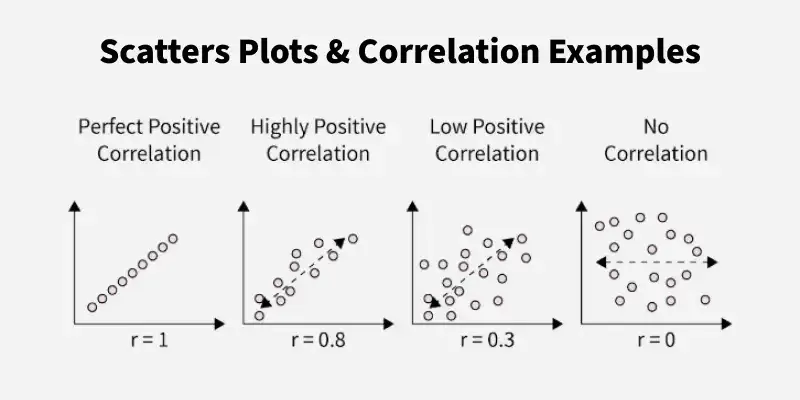 Scatter plots showing correlation
Karl Pearson's Coefficient and Spearman’s Rank Correlation
When analyzing relationships between variables, it is important to choose the right correlation method based on the type of data and its distribution. Two widely used methods are Karl Pearson's Coefficient of Correlation and Spearman’s Rank Correlation.
1. Karl Pearson's Coefficient: This is the most common method to calculate correlation. It provides a standardized value (ranging from -1 to +1) that indicates both the direction (positive or negative) and the strength of the relationship. This method assumes that the data follows a normal distribution and that the relationship between variables is linear.
It is also a default method to find correlation in many programming languages using the formula:
r=∑(X−Xˉ)(Y−Yˉ)∑(X−Xˉ)2⋅∑(Y−Yˉ)2
r=∑(X−X
ˉ
)2
⋅∑(Y−Y
ˉ
)2
∑(X−X
ˉ
)(Y−Y
ˉ
)
where Xˉ
X
ˉ
and Yˉ
Y
ˉ
are the means of X and Y.
- It only works for linear relationships.
- Sensitive to outliers, which can distort results.
- Assumes normality in data distribution.
2. Spearman’s Rank Correlation : It is used when data does not follow a normal distribution or when dealing with ordinal data (data that can be ranked but not measured precisely). Unlike Pearson’s correlation, Spearman’s method measures the strength and direction of a monotonic relationship, meaning that as one variable increases, the other consistently increases or decreases, even if the relationship is not linear. The formula is:
ρ=1−6∑di2n(n2−1)
ρ=1−n(n2
−1)
6∑di
2
where di
di is the difference between the ranks of X and Y and n is the total number of observations.
Both methods are essential tools in data science:
- Karl Pearson's Coefficient is ideal for analyzing continuous variables with linear relationships.
- Spearman’s Rank Correlation is better suited for non-linear or ranked data.
Limitations of Covariance and Correlation
Covariance:
- Covariance depends on the units used making it hard to interpret if the variables are measured in different units.
- It only works for straight-line relationships and doesn’t capture more complex or curved relationships.
- Covariance doesn’t show how strong the relationship.
Correlation:
- Correlation assumes a straight-line relationship and doesn’t work well with non-linear relationships.
- Correlation can be heavily affected by outliers.
- Correlation is best for normally distributed data and may not be reliable for skewed data.
- with the target variable, improving model accuracy.