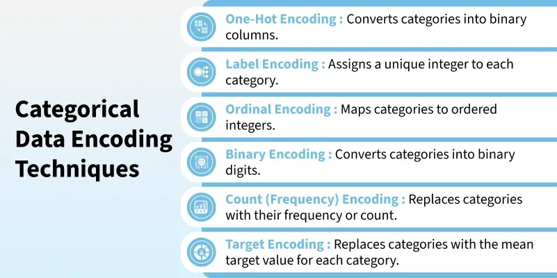
Categorical Data Encoding Techniques in Machine Learning

Categorical data refers to variables that belong to distinct categories such as labels, names or types. Since most machine learning algorithms require numerical inputs, encoding categorical data to numerical data becomes important. Proper encoding ensures that models can interpret categorical variables effectively, leading to improved predictive accuracy and reduced bias.

Types of Categorical Data

1. Nominal Data: Nominal data consists of categories without any inherent order or ranking. These are simple labels used to classify data.

• Example: 'Red', 'Blue', 'Green' (Car Color).
• Encoding Options: One-Hot Encoding or Label Encoding, depending on the model's needs.

2. Ordinal Data: Ordinal data includes categories with a defined order or ranking, where the relationship between values is important.

• Example: 'Low', 'Medium', 'High' (Car Engine Power).
• Encoding Options: Ordinal Encoding.

Using the right encoding techniques, we can effectively transform categorical data for machine learning models which improves their performance and predictive capabilities.

Techniques to perform Categorical Data Encoding

Techniques

1. Label Encoding

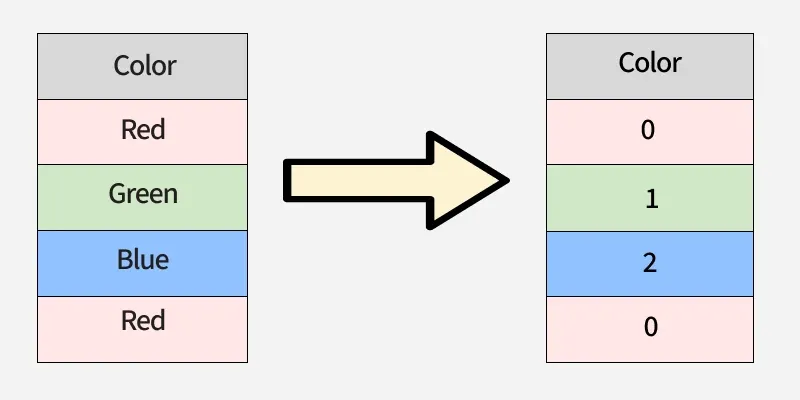
Label Encoding assigns each category a unique integer. It is simple and memory-efficient but may unintentionally imply an order among categories when none exists.

• Used in tree-based models like Decision Trees or XGBoost.
• Pros: Simple and memory-efficient.
• Cons: Introduces implicit order which may be misinterpreted by non-tree models when used with nominal data.

Label Encoding

Let's look at the following example:

from sklearn.preprocessing import LabelEncoder

data = ['Red', 'Green', 'Blue', 'Red']

le = LabelEncoder()
encoded_data = le.fit_transform(data)
print(f"Encoded Data: {encoded_data}")

Output:

Encoded Data: [0 1 2 0]

Here, 'Red' becomes 0, 'Green' becomes 1 and 'Blue' becomes 2.

2. One-Hot Encoding

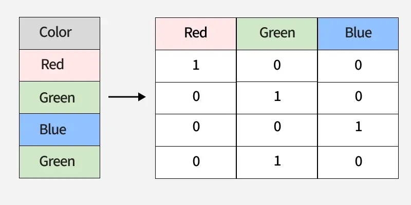
One-Hot Encoding converts categories into binary columns with each column representing one category. It prevents false ordering but can lead to high dimensionality if there are many unique values.

• Used in linear models, logistic regression and neural networks.
• Pros: Does not assume order; widely supported.
• Cons: Can cause high dimensionality and sparse data when feature has many categories.

One-Hot Encoding

Let's look at the following example:

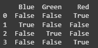
import pandas as pd

data = ['Red', 'Blue', 'Green', 'Red']

df = pd.DataFrame(data, columns=['Color'])
one_hot_encoded = pd.get_dummies(df['Color'])

print(one_hot_encoded)

Output:

output

Each unique category ('Red', 'Blue', 'Green') is transformed into a separate binary column, with 1 representing the presence of the category and 0 its absence.

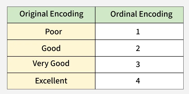
3. Ordinal Encoding

Ordinal Encoding maps categories to integers while preserving their natural order. This works well for ordered data like ratings but is not suitable for nominal variables.

• Used for ordered features like ratings or education levels.
• Pros: Maintains order; reduces dimensionality.
• Cons: Not suitable for nominal categories.

Ordinal Encoding

Let's consider the following example:

from sklearn.preprocessing import OrdinalEncoder
data = [['Low'], ['Medium'], ['High'], ['Medium'], ['Low']]

encoder = OrdinalEncoder(categories=[['Low', 'Medium', 'High']])
encoded_data = encoder.fit_transform(data)

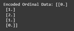
print(f"Encoded Ordinal Data: {encoded_data}")

Output:

output

In this case, 'Low' is encoded as 0, 'Medium' as 1 and 'High' as 2, preserving the natural order of the categories.

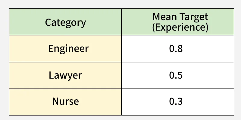
4. Target Encoding

Target Encoding also known as Mean Encoding is a technique where each category in a feature is replaced by the mean of the target variable for that category.

• Useful for high-cardinality features like ZIP codes or product IDs.
• Pros: Captures relationship to target variable.
• Cons: Risk of overfitting, also must apply smoothing/statistical techniques.

Target Encoding

Let's consider the following example:

import pandas as pd
import category_encoders as ce

df = pd.DataFrame(
    {'City': ['London', 'Paris', 'London', 'Berlin'], 'Target': [1, 0, 1, 0]}
)

encoder = ce.TargetEncoder(cols=['City'])
df_tgt = encoder.fit_transform(df['City'], df['Target'])

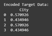
print(f"Encoded Target Data:\n{df_tgt}")

Output:

output

In this case, each color is encoded based on the mean of the target variable. For instance, 'Red' has a mean target value of approximately 0.485, which reflects the target values for the rows where 'Red' appears.

5. Binary Encoding

Binary encoding represents categories as binary codes and splits them across multiple columns. It is efficient for high-cardinality data but slightly more complex to implement.

• Applied in high-cardinality text/NLP tasks to save memory.
• Pros: Reduces dimensionality, more memory-efficient than one-hot encoding.
• Cons: Slightly more complex; requires careful handling of missing values.

Binary Encoding

Let's consider the following example:

import category_encoders as ce
data = ['Red', 'Green', 'Blue', 'Red']
encoder = ce.BinaryEncoder(cols=['Color'])
encoded_data = encoder.fit_transform(pd.DataFrame(data, columns=['Color']))
print(encoded_data)

Output:

output

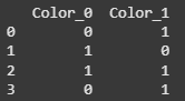
Here, each category (like 'Red', 'Blue', 'Green') is converted into binary digits. 'Red' gets the binary code '10', 'Blue' becomes '01' and 'Green' becomes '11'. Each binary digit is placed in a separate column (e.g., Color_0 and Color_1).

6. Frequency Encoding

Frequency Encoding assigns categories values based on how often they occur in the dataset. It is simple and compact but can introduce data leakage if applied improperly.

• Effective in retail, e-commerce or clickstream data for popularity trends.
• Pros: Low computational and storage requirements.
• Cons: Can introduce data leakage if not handled properly.

Frequency Encoding

Let's consider the following example:

import pandas as pd
data = ['Red', 'Green', 'Blue', 'Red', 'Red']
series_data = pd.Series(data)
frequency_encoding = series_data.value_counts()

encoded_data = [frequency_encoding[x] for x in data]
print("Encoded Data:", encoded_data)

Output:

Encoded Data: [np.int64(3), np.int64(1), np.int64(1), np.int64(3), np.int64(3)]

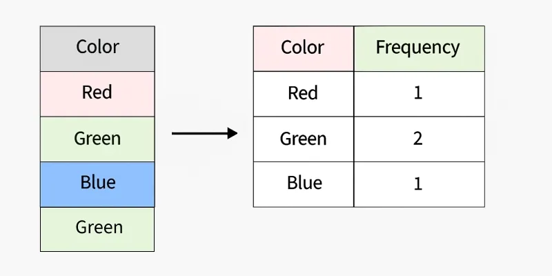
Here, 'Red' appears 3 times, so it is encoded as 3, while 'Green' and 'Blue' appear once, so they are encoded as 1.

Differences between Various Techniques

TechniqueSuitable ForDimensionalityOverfitting RiskInterpretabilityOne-Hot EncodingNominalHighLowHighLabel EncodingOrdinal (sometimes Nominal)LowMediumMediumOrdinal EncodingOrdinalLowMediumHighBinary EncodingHigh-cardinality featuresMediumMediumMediumFrequency EncodingHigh-cardinalityLowHighMediumTarget EncodingHigh-cardinalityLowHighLow-Medium